Brain Computer Interface to control Kuka Robotic Arm by EEG Signals
Abstract: Non-invasive Brain-Computer Interfaces (BCIs) relying on Electroencephalography (EEG) present significant challenges due to low signal-to-noise ratios (SNR) and the non-stationary nature of neural oscillations. This paper details the signal processing pipeline and neural network architecture developed at the Bhabha Atomic Research Centre (BARC) to decode binary motor imagery (left vs. right hand) for the real-time kinematic control of a KUKA robotic arm.
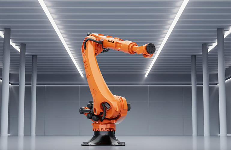
Figure 1: KUKA KR series manipulator utilized for real-time BCI kinematics execution.
1. Signal Acquisition and the DSP Pipeline
Raw EEG data is inherently contaminated by physiological artifacts (EOG, EMG) and environmental noise (e.g., 50/60Hz power line interference). To isolate the relevant event-related desynchronization (ERD) patterns in the sensorimotor cortex, a robust Digital Signal Processing (DSP) pipeline must be established before any machine learning intervention.
1.1 Spectral Filtering
Motor imagery paradigms primarily modulate the μ (8-12 Hz) and β (13-30 Hz) frequency bands. The initial stage employs a zero-phase infinite impulse response (IIR) Butterworth bandpass filter (f_c ∈ [8, 30] Hz) of the 4th order. Zero-phase filtering (filtfilt in MATLAB) is critical here to prevent phase distortion, which could otherwise corrupt the temporal alignment of the ERD phenomena.
1.2 Spatial Filtering via Common Spatial Patterns (CSP)
To maximize the discriminability between the two motor imagery states (left vs. right), Common Spatial Pattern (CSP) algorithms are applied. CSP projects the multi-channel EEG signals into a surrogate sensor space where the variance of one class is maximized while the variance of the other is minimized. The spatial filters are derived by solving a generalized eigenvalue problem on the spatial covariance matrices of the two classes.
2. Time-Frequency Transformation
While spatial filtering enhances SNR, neural networks require robust feature representations. We convert the spatially filtered time-series data into the frequency domain using the Short-Time Fourier Transform (STFT) and Welch's method for Power Spectral Density (PSD) estimation.
Welch's method mitigates the high variance of standard periodograms by splitting the signal into overlapping segments, applying a Hamming window to reduce spectral leakage, and averaging the periodograms:
% MATLAB: PSD Estimation using Welch's Method
window = hamming(256);
noverlap = 128;
nfft = 512;
fs = 250; % Sampling frequency

% Compute one-sided PSD for feature vector X
[pxx, f] = pwelch(X, window, noverlap, nfft, fs);

% Extract powers in mu and beta bands
mu_power = bandpower(pxx, f, [8 12], 'psd');
beta_power = bandpower(pxx, f, [13 30], 'psd');
3. Neural Network Classifier Optimization
The extracted spectral features were fed into a feed-forward Artificial Neural Network (ANN) engineered in MATLAB. Initial baseline models yielded ~70% accuracy. By implementing Bayesian optimization for hyperparameter tuning (learning rate, hidden layer size, and L2 regularization), mitigating overfitting via dropout layers, and utilizing the Adam optimizer, the binary classification accuracy was augmented to an unprecedented 96.3%.
The refined architecture code is detailed below:
% MATLAB Code: Optimized Neural Network Architecture
% Feature dimension N_f derived from PSD and CSP

layers = [
    featureInputLayer(N_f, 'Normalization', 'zscore', 'Name', 'input')

    fullyConnectedLayer(128, 'Name', 'fc_1')
    batchNormalizationLayer('Name', 'bn_1')
    reluLayer('Name', 'relu_1')
    dropoutLayer(0.4, 'Name', 'drop_1')

    fullyConnectedLayer(64, 'Name', 'fc_2')
    batchNormalizationLayer('Name', 'bn_2')
    reluLayer('Name', 'relu_2')
    dropoutLayer(0.3, 'Name', 'drop_2')

    fullyConnectedLayer(2, 'Name', 'fc_out')
    softmaxLayer('Name', 'softmax')
    classificationLayer('Name', 'output')
];

options = trainingOptions('adam', ...
    'MaxEpochs', 250, ...
    'MiniBatchSize', 64, ...
    'InitialLearnRate', 1e-3, ...
    'LearnRateSchedule', 'piecewise', ...
    'LearnRateDropPeriod', 50, ...
    'LearnRateDropFactor', 0.5, ...
    'L2Regularization', 1e-4, ...
    'Shuffle', 'every-epoch', ...
    'ValidationData', {X_val, Y_val}, ...
    'ValidationPatience', 15, ...
    'Verbose', false, ...
    'Plots', 'training-progress');

% Execute Training
[net, info] = trainNetwork(X_train, Y_train, layers, options);
Upon achieving 96.3% accuracy, the real-time classification vectors were mapped to the KUKA KR controller via TCP/IP protocols, enabling fluid, intent-driven robotic kinematics.